Define data analysis parameters¶

A multitude of different analysis methods and visualisation plots have been implemented within the analytics_core of the Clinical Knowledge Graph. The table below contains the current list of methods and visualizations available:

Table CKG Analytics Core

	Step	Method	Description	CKG function	Reference	Link
Data preparation	Power analysis	anova power analysis	Determine the sample size required to detect an effect of a given size with a given degree of confidence	power_analysis	https://machinelearningmastery.com/statistical-power-and-power-analysis-in-python/	https://www.statsmodels.org/stable/generated/statsmodels.stats.power.FTestAnovaPower.html
	Filtering	percentage	Filtering based on maximum percentage of missing values allowed (per group optional)	extract_percentage_missing
	Filtering	at_least_x	Filtering based on minimum number of present values (per group optional)	extract_number_missing
	Imputation	K-nearest Neighbors	Imputation based on the algorithm Nearest Neighbors (NN)	imputation_KNN	https://www.ncbi.nlm.nih.gov/pubmed/21743766	https://pypi.org/project/fancyimpute/
		Probabilistic Minimum Imputation approach	Imputation method replacing missing values with values withdrawn from a down-shifted normal distribution	imputation_normal_distribution	https://www.ncbi.nlm.nih.gov/pubmed/26906401
		Mixed model	A combination of KNN and Probabilistic Minimum depending on the number of values available (>60% KNN, rest ProbMin)	imputation_mixed_norm_KNN
	Normalization	Median	Normalize samples using the median	median_normalization
		Median polish	Normalization based on the medians obtained from the rows and the columns to iteratively calculate the row effect and column effect on the data	median_polish_normalization
		Quantile	Adjustment method that forces the observed distributions to be the same and it uses the average of each quantile across samples as the reference (assumes the statistical distribution of each sample is the same)	quantile_normalization
		Linear	Apply l1 or l2 normalization	linear_normalization		https://scikit-learn.org/stable/modules/preprocessing.html
	Batch effect correction	COMBAT	Adjust for batch effects in datasets where the batch covariate is known	combat_batch_correction	https://pubmed.ncbi.nlm.nih.gov/16632515/	https://github.com/epigenelabs/pyComBat
Data exploration	Ranking	Ranking	Ranking of proteins based on intensity	get_ranking_with_markers
	Coefficient of Variation	Coefficient of Variation	Coefficient of variation per group as a quality control	get_coefficient_variation
	QC markers	QC Makers	If there are quality control markers associated with the tissue studied, they are used to visualize possible outliers (z-score) among the samples	run_qc_markers_analysis	https://www.ncbi.nlm.nih.gov/pubmed/31566909
	Summary statistics	Summary statistics	Statistics for rows and columns in the data matrix	get_summary_data_matrix
Data analysis	Dimensionality reduction	PCA	Principal Component Analysis (2D, 3D)	run_pca	https://www.ncbi.nlm.nih.gov/pubmed/24061923	https://scikit-learn.org/stable/modules/generated/sklearn.decomposition.PCA.html
		tSNE	t-distributed Stochastic Neighbor Embedding	run_tsne	https://www.ncbi.nlm.nih.gov/pubmed/30252473	https://scikit-learn.org/stable/modules/generated/sklearn.manifold.TSNE.html
		UMAP	Uniform Manifold Approximation and Projection	run_umap	https://arxiv.org/abs/1802.03426	https://umap-learn.readthedocs.io/
	Hypothesis testing	SAMR	Significance analysis of microarrays applied to proteomics data	run_samr	https://www.ncbi.nlm.nih.gov/pubmed/11309499	https://www.rdocumentation.org/packages/samr/versions/3.0
		ANOVA	Analysis of Variance	run_anova		https://pingouin-stats.org/generated/pingouin.anova.html
		ANOVA-rm	Analysis of Variance for repeated measurements	run_repeated_measurements_anova		https://pingouin-stats.org/generated/pingouin.rm_anova.html
		t-test	t-test mean difference	run_ttest		https://pingouin-stats.org/generated/pingouin.ttest.html
	Multiple-test correction	Bonferroni	Bonferroni p-value correction	apply_pvalue_correction		https://www.statsmodels.org/stable/generated/statsmodels.stats.multitest.multipletests.html
		Benjamini-Hochberg	Benjamini-Hochberg FDR correction	apply_pvalue_correction		https://www.statsmodels.org/stable/generated/statsmodels.stats.multitest.multipletests.html
		Permutation-FDR	Permutation FDR	apply_pvalue_permutation_fdrcorrection	https://www.jstor.org/stable/2346101
		…	…	apply_pvalue_correction		https://www.statsmodels.org/stable/generated/statsmodels.stats.multitest.multipletests.html
	Correlation	Correlation	Pearson or Spearman correlation	run_correlation
	Correlation	Correlation-rm	Pearson or Spearman correlation for repeated measurements	run_rm_correlation		https://pingouin-stats.org/generated/pingouin.rm_corr.html
	Enrichment	Single Sample Gene Set Enrichment Analysis	Single-sample GSEA (ssGSEA), an extension of Gene Set Enrichment Analysis (GSEA), calculates separate enrichment scores for each pairing of a sample and gene set. Each ssGSEA enrichment score represents the degree to which the genes in a particular gene set are coordinately up- or down-regulated within a sample. (https://www.genepattern.org/modules/docs/ssGSEAProjection/4)	run_ssgsea	https://pubmed.ncbi.nlm.nih.gov/16199517/	https://github.com/zqfang/gseapy
	Enrichment	Fisher Exact Test	Significant test for contingency tables	run_enrichment		https://docs.scipy.org/doc/scipy/reference/generated/scipy.stats.fisher_exact.html
	Network analysis	Louvain partition	Best partition algorithm	get_louvain_partitions	https://www.ncbi.nlm.nih.gov/pubmed/21517554	https://python-louvain.readthedocs.io/en/latest/api.html
		Greedy modularity	A hierarchical agglomeration algorithm for detecting community structure	get_network_communities	https://www.ncbi.nlm.nih.gov/pubmed/15697438	https://networkx.github.io/documentation/stable/reference/algorithms/generated/networkx.algorithms.community.modularity_max.greedy_modularity_communities.html
		Asynchronous label propagation algorithm	The algorithm initializes each node with a unique label and repeatedly sets the label of a node to be the label that appears most frequently among that nodes neighbors. The algorithm halts when each node has the label that appears most frequently among its neighbors	get_network_communities	https://www.ncbi.nlm.nih.gov/pubmed/17930305	https://networkx.github.io/documentation/stable/reference/algorithms/generated/networkx.algorithms.community.label_propagation.asyn_lpa_communities.html#id3
		Girvan-Newman algorithm	Hierachical algorithm that removes edges iteratively and defining communities by the remaining connected components	get_network_communities		https://networkx.github.io/documentation/stable/reference/algorithms/generated/networkx.algorithms.community.centrality.girvan_newman.html
		Affinity propagation	A centroid-based clustering algorithm that finds members of the input set that are representative of clusters and estimates the number of clusters	get_network_communities	https://www.ncbi.nlm.nih.gov/pubmed/17218491	https://scikit-learn.org/stable/modules/generated/sklearn.cluster.affinity_propagation.html
		Similarity Network Fusion	SNF computes and fuses patient similarity networks obtained from each of their data types separately, taking advantage of the complementarity in the data.	run_snf	https://pubmed.ncbi.nlm.nih.gov/24464287/	https://snfpy.readthedocs.io/en/latest/
	Multiomics	WGCNA	Weighted gene co-expression network analysis for describing the correlation patterns among proteinsfinding clusters (modules) of highly correlated genes, for summarizing such clusters using the module eigengene or an intramodular hub gene, for relating modules to one another and to external sample traits	run_WGCNA	https://www.ncbi.nlm.nih.gov/pubmed/19114008	https://horvath.genetics.ucla.edu/html/CoexpressionNetwork/Rpackages/WGCNA/
Visualization	Viz	Pie chart	Circular statistical chart, which is divided into sectors to illustrate numerical proportion	get_pieplot		https://plotly.com/python/pie-charts/
		Distribution plot	Representations of statistical distributions	get_distplot		https://plotly.com/python/distplot/
		Bar chart		get_barplot		https://plotly.com/python/bar-charts/
		Scatter plot matrix		get_facet_grid_plot
		Ranking plot		get_ranking_plot
		Scatter plot		get_simple_scatterplot
		Volcano plot		run_volcano
		Heatmap plot		get_heatmapplot
		Heatmap plot with annotation and clustering		get_complex_heatmapplot
		Network	Generates a Cytoscape network (Plot.ly), a Jupyter notebook compatible Cytoscape network (Cyjupyter) and a json format network	get_network	https://www.ncbi.nlm.nih.gov/pubmed/14597658	https://dash.plotly.com/cytoscape
		PCA plot	PCA plot with loadings (2D and 3D)	get_pca_plot
		Sankey diagram	Visualize the contributions to a flow	get_sankey_plot
		Table		get_table		https://dash.plotly.com/datatable
		Violin plot		get_violinplot		https://plotly.com/python/violin/
		Parallel coordinates plot		get_parallel_plot		https://plotly.com/python/parallel-coordinates-plot/
		WGCNA plots	Generates all the plots for the WGCNA analysis	get_WGCNAPlots	https://www.ncbi.nlm.nih.gov/pubmed/19114008	https://horvath.genetics.ucla.edu/html/CoexpressionNetwork/Rpackages/WGCNA/
		2-way Venn diagram		get_2_venn_diagram		https://plotly.com/python/shapes/
		Word cloud	Represents the frequency of words in a text using size and color	get_wordcloud		https://github.com/PrashantSaikia/Wordcloud-in-Plotly
		Save Dash plot	Save a Dash figure object to svg format	save_DASH_plot
		Kaplan-meier plot	Kaplan-meier survival plot with significance annotation	get_km_plot		https://plotly.com/python/v3/ipython-notebooks/survival-analysis-r-vs-python/
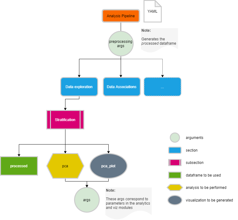
		Polar chart	Represents data along radial and angular axes	get_polar_plot		https://plotly.com/python/polar-chart/

The default workflow makes use of the functions defined in this module and runs, for each data type, the analysis pipeline defined in a configuration file. These configuration files are defined in YAML format (https://yaml.org/spec/1.2/spec.html), which can be easily read in Python into a dictionary structure with sections and analyses. For each analysis we need to define the data that will be used (i.e original data), how the results will be visualized (i.e pca_plot) and what parameters need to be used (i.e components: 2).

In the CKG, we have default analyses defined for clinical, proteomics, phosphoproteomics and interactomics datasets. All the analysis configuration files can be modified to fit your project or data. To check how each configuration files look like and how to modify them, please follow the links below and also review the specific functions in CKG’s API Reference to define the args to use.

Data configuration files

Adding New Analyses or visualizations¶

If you would like to contribute to CKG and add new analysis or visualization functions you can implement them in the Analytics or Viz modules respectively. To make your new analysis or visualization available as part of the default analytical pipeline, you will need to add a conditional block in the analytics_factory.py module. For instance:

elif self.analysis_type == "NEW_ANALYSIS":
   arg1 = 'VALUE'
   arg2 = 'VALUE'
   arg3 = 'VALUE'
   if "arg1" in self.args:
      arg1 = self.args["arg1"]
   if "arg2" in self.args:
      arg2 = self.args["arg2"]
   if "arg3" in self.args:
      arg3 = self.args["arg3"]
   self.result[self.analysis_type] = analytics.run_new_function(self.data, arg1=arg1, arg2=arg2, arg3=arg3)

To incorporate this new analysis into the configuration file just add a new section, for example:

new analysis section:
   new analysis subsection:
      description: 'This is a new function in the analytics core'
      data: processed
      analyses:
         - NEW_ANALYSIS
      plots:
         - scatterplot
      args:
         arg1: 'value1'
         arg2: 'value2'
         arg3: 'value3'
         x_title: 'x axis'
         y_title: 'y axis'
         width: 1000
         height: 700
         title: 'Scatter plot for my new analysis'

Finally, just add the new function to the table here in the docs :)!